【科学技術計算講座4-9】有限体積法プログラミング~2次元熱伝導問題

前回は有限体積法の線形方程式を解く共役勾配法という解法について説明しました。

線形方程式系の解法である共役勾配法について解説します。また線形方程式系を行列で表し、その行列の特徴である対称疎行列について説明します。科学技術計算講座4「有限体積法で熱伝導シミュレーション」の第8回目です。

今回はシリーズ最終回です。共役勾配法をPythonでプログラミングして有限体積法のプログラムを完成させたいと思います。

共役勾配法のプログラム

前回説明したとおり共役勾配法のアルゴリズムは以下のとおりです。

  1.  適当な初期値 ${\bf T}_0$ を決める。
  2.  ${\bf r}_0 = {\bf b} - {\bf A} {\bf T}_0$、 ${\bf d}_0 = {\bf r}_0$  とする。
  3.  収束するまで以下の計算を繰り返す。
    ① $\alpha_k=({\bf d}_k, {\bf r}_k)/({\bf d}_k, {\bf A}{\bf d}_k) $ 
    ② ${\bf T}_{k+1} = {\bf T}_k + \alpha_k {\bf d}_k$ 
    ③ ${\bf r}_{k+1} = {\bf r}_k - \alpha_k{\bf A} {\bf d}_k$ 
    ④ 残差 ${\bf r}_{k+1}$ で収束判定。収束なら終了。
    ⑤ $\beta_k= ({\bf r}_{k+1}, {\bf r}_{k+1})/({\bf r}_k, {\bf r}_k)$ 
    ⑥ ${\bf d}_{k+1} = {\bf r}_{k+1} + \beta_k {\bf d}_k $ 

今回の有限体積法でのPythonプログラムは以下のようになります。

プログラムの表示
itermax = 1000
eps = 1.0e-5

d = np.zeros_like(temp)
r = np.zeros_like(temp)
ad = np.zeros_like(temp)

#-- initial residual
for icell in range(1, ncell+1):
    r[icell] = bc[icell] - ac[icell] * temp[icell]
    for iface in range(4):
        inbor = cnbor[icell][iface]
        r[icell] -= af[icell][iface] * temp[inbor]  
d = np.copy(r)
rr = np.dot(r, r)
bnrm = np.linalg.norm(bc)

#-- iteration
for iter in range(1, itermax+1):
    #-- A*d
    for icell in range(1, ncell+1):
        ad[icell] = ac[icell] * d[icell]
        for iface in range(4):
            inbor = cnbor[icell][iface]
            ad[icell] += af[icell][iface] * d[inbor]     

    #-- alpha                    
    alpha = np.dot(d, r) / np.dot(d, ad)

    #-- temperature
    temp += alpha * d

    #-- residual
    r -= alpha * ad    
    resd = np.linalg.norm(r) / bnrm

    #-- convergence check
    if resd <= eps:
        break  

    #-- beta
    beta = np.dot(r, r) / rr
    rr = np.dot(r, r)

    #-- d
    d = r + beta * d
d = np.zeros_like(temp)
r = np.zeros_like(temp)
ad = np.zeros_like(temp)

まず配列を用意します。d は方向ベクトル ${\bf d}$、r は残差ベクトル ${\bf r}$、ad は行列 ${\bf A}$ と ${\bf d}$ の積 ${\bf A}{\bf d}$ です。

#-- initial residual
for icell in range(1, ncell+1):
    r[icell] = bc[icell] - ac[icell] * temp[icell]
    for iface in range(4):
        inbor = cnbor[icell][iface]
        r[icell] -= af[icell][iface] * temp[inbor]  

ここは、残差ベクトルの初期値 ${\bf r}_0 = {\bf b} - {\bf A} {\bf T}_0$ を計算しています。

d = np.copy(r)
rr = np.dot(r, r)
bnrm = np.linalg.norm(bc)

d = np.copy(r) は ${\bf d}_0 = {\bf r}_0$ で、rd にコピーしています。

rr = np.dot(r, r) は、rr の内積を計算しています。あとで $\beta$ を計算するときに使います。

bnrm = np.linalg.norm(bc) は、bc のノルム $||{\bf b}||$ を計算しています。相対残差を計算するときに使います。

#-- iteration
for iter in range(1, itermax+1):

共役勾配法の反復計算のforループです。iter は反復回数で 1 から itermax まで回ります。

    #-- A*d
    for icell in range(1, ncell+1):
        ad[icell] = ac[icell] * d[icell]
        for iface in range(4):
            inbor = cnbor[icell][iface]
            ad[icell] += af[icell][iface] * d[inbor]     

${\bf A}{\bf d}$ を計算しています。

    #-- alpha                    
    alpha = np.dot(d, r) / np.dot(d, ad)

$\alpha$ を計算します。

    #-- temperature
    temp += alpha * d

温度 ${\bf T}$ を更新します。

    #-- residual
    r -= alpha * ad    
    resd = np.linalg.norm(r) / bnrm

残差ベクトル ${\bf r}$ を更新して、相対残差 $||{\bf r}||/||{\bf b}||$ を計算します。

    #-- convergence check
    if resd <= eps:
        break  

収束判定をチェックします。残差 resd が収束判定値 eps 以下になると、break で反復のforループを抜けます。

eps は最初に定義している小さな数です。今回は 1.0e-5 としています。残差がどのくらいになれば収束とみなすかは、実際の問題では厳密な指標を示すのは難しいです。収束判定値 eps が大きいと収束が早いですが、定常状態になっていない場合があります。逆に eps が小さいと真の解により近づきますが、収束までの反復回数が多くなり計算時間がかかります。計算結果やあとで紹介するモニター点の履歴などを見ながら収束を総合的に判断する必要があります。

    #-- beta
    beta = np.dot(r, r) / rr
    rr = np.dot(r, r)

    #-- d
    d = r + beta * d

最後に $\beta$ を計算し、${\bf d}$ を更新します。rr は次のステップ用に rr の内積を格納しています。

共役勾配法のアルゴリズムはシンプルなので、プログラムもアルゴリズムの通りでとてもシンプルに書けます。

2次元熱伝導問題の有限体積法プログラム

以上でプログラムの骨格は出来たので、今回の2次元熱伝導問題の有限体積法プログラムの完成版を載せておきます。

プログラムの表示
import numpy as np
import matplotlib.pyplot as plt

# input parameter =====================================================
#-- geometry
lx = 1.0
ly = 1.0
nx = 50
ny = 50

dx = lx / nx
dy = ly / ny 
ncell = nx * ny 

#-- solver
itermax = 1000
eps = 1.0e-5

#-- monitor
pmon = np.array([0.5, 0.5])

# condition ====================================================
#-- temperature
temp = np.full(ncell+1, 300.0)

#-- thermal conductivity
cond = np.full_like(temp, 100.0)
for i in range(1, nx+1):
    for j in range(1, ny+1):
        icell = i + (j - 1) * nx
        x = (i - 0.5) * dx
        y = (j - 0.5) * dy
        if y >= 0.8:
            cond[icell] = 10.0

#-- heat source
qc = np.zeros_like(temp)

#-- find monitor cell
imon = 0
flag = False
for i in range(1, nx+1):
    for j in range(1, ny+1):
        icell = i + (j - 1) * nx
        x = (i - 1) * dx
        y = (j - 1) * dy
        if pmon[0] >= x and pmon[0] <= (x+dx) and pmon[1] >= y and pmon[1] <= (y+dy):
            imon = icell
            flag = True
            break
    if flag:
        break          

# algebraic equations ==============================================  
def boundary(icell, iface, btype, tb=300.0, qb=0.0, ta=300.0, ht=10.0):
    condf = cond[icell]
    dcb = 0.5 * dcf[iface]

    if btype == 'dirichlet': # Dirichlet
        a_b = -condf * s[iface] / dcb
        a_f = 0.0
        a_c = -a_b
        b_c = -a_b * tb
    elif btype == 'neumann': # Neumann
        a_f = 0.0
        a_c = 0.0
        b_c = -qb * s[iface]
    elif btype == 'mixed': # Mixed                     
        htc = condf / dcb
        htf = ht * htc / (ht + htc) 
        a_b = -htf * s[iface] 
        a_f = 0.0
        a_c = -a_b
        b_c = -a_b * ta   

    return a_f, a_c, b_c  
    
s = [dy, dy, dx, dx]
dcf = [dx, dx, dy, dy] 
volume = dx * dy

ac = np.zeros_like(temp)
af = np.zeros((ncell+1, 4))
bc = np.zeros_like(temp)
cnbor = np.zeros_like(af, dtype='int')

for i in range(1, nx+1):
    for j in range(1, ny+1):
        icell = i + (j - 1) * nx
        x = (i - 0.5) * dx
        y = (j - 0.5) * dy

        ac[icell] = 0.0
        bc[icell] = qc[icell] * volume

        #-- face loop
        for iface in range(4):

            #-- face type
            if iface == 0 and i == nx: 
                ftype = 'right'
            elif iface == 1 and i == 1: 
                ftype = 'left'
            elif iface == 2 and j == ny: 
                ftype = 'top'
            elif iface == 3 and j == 1: 
                ftype = 'bottom'
            else:
                ftype = 'internal'
            
            #-- neighbor cell
            if ftype == 'internal':
                if iface == 0: inbor = icell + 1 # East
                elif iface == 1: inbor = icell - 1 # West
                elif iface == 2: inbor = icell + nx # North
                elif iface == 3: inbor = icell - nx # South
            else:
                inbor = 0    
            cnbor[icell][iface] = inbor                
            
            #-- matrix
            if ftype == 'internal': # internal face
                gf = 0.5
                condf = cond[icell] * cond[inbor] / ((1.0 - gf) * cond[icell] + gf * cond[inbor])
                a_f = -condf * s[iface] / dcf[iface]
                a_c = -a_f
                b_c = 0.0
            else: # boundary face
                if ftype == 'right' and y <= 0.2:
                    a_f, a_c, b_c = boundary(icell, iface, 'dirichlet', tb=500.0)
                elif ftype == 'top' and x <= 0.5: 
                    a_f, a_c, b_c = boundary(icell, iface, 'dirichlet', tb=300.0)  
                elif ftype == 'left':
                    a_f, a_c, b_c = boundary(icell, iface, 'mixed', ta=400.0, ht=100.0)
                else:
                    a_f, a_c, b_c = boundary(icell, iface, 'neumann', qb=0.0)

            ac[icell] += a_c
            af[icell][iface] = a_f
            bc[icell] += b_c   

# CG solver ===================================================      
iter_plt = []
resd_plt = []
temp_plt = []
d = np.zeros_like(temp)
r = np.zeros_like(temp)
ad = np.zeros_like(temp)

#-- initial residual
for icell in range(1, ncell+1):
    r[icell] = bc[icell] - ac[icell] * temp[icell]
    for iface in range(4):
        inbor = cnbor[icell][iface]
        r[icell] -= af[icell][iface] * temp[inbor]  
d = np.copy(r)
rr = np.dot(r, r)
bnrm = np.linalg.norm(bc)

#-- iteration
for iter in range(1, itermax+1):
    #-- A*d
    for icell in range(1, ncell+1):
        ad[icell] = ac[icell] * d[icell]
        for iface in range(4):
            inbor = cnbor[icell][iface]
            ad[icell] += af[icell][iface] * d[inbor]     

    #-- alpha                    
    alpha = np.dot(d, r) / np.dot(d, ad)

    #-- temperature
    temp += alpha * d

    #-- residual
    r -= alpha * ad    
    resd = np.linalg.norm(r) / bnrm

    #-- plot data
    iter_plt.append(iter)
    resd_plt.append(resd)
    temp_plt.append(temp[imon])
    print('iter {:6d} , resd {:12.4e} , temp {:12.4e}'.format(iter, resd, temp[imon]))

    #-- convergence check
    if resd <= eps:
        break  

    #-- beta
    beta = np.dot(r, r) / rr
    rr = np.dot(r, r)

    #-- d
    d = r + beta * d

# post processing ====================================================
#-- residual and monitor graph
fig1 = plt.figure()
ax1 = fig1.add_subplot(2, 1, 1)
ax1.plot(iter_plt, resd_plt)
ax1.set(ylabel='Residual')
ax1.set_yscale('log')

ax2 = fig1.add_subplot(2, 1, 2)
ax2.plot(iter_plt, temp_plt)
ax2.set(xlabel='Iteration', ylabel='Monitor')      

#-- contour plot
fig2 = plt.figure()
ax3 = fig2.add_subplot(1, 1, 1)

gx = np.arange(0.0, lx+0.5*dx, dx)
gy = np.arange(0.0, ly+0.5*dy, dy)
X, Y = np.meshgrid(gx, gy)

val = np.zeros((ny, nx))
for i in range(1, nx+1):
    for j in range(1, ny+1):
        icell = i + (j - 1) * nx 
        val[j-1][i-1] = temp[icell]

im = ax3.pcolormesh(X, Y, val, cmap='jet')
ax3.set_xlabel('x')
ax3.set_ylabel('y')
ax3.set_aspect('equal')
fig2.colorbar(im)
plt.show()

→プログラムはこちら(GitHub)

以下はプログラムの補足です。

モニター点の表示

今回の問題では板の中央の温度を知りたいとありました。そこで、指定した位置の値を画面に表示することにします。有限体積法はセルごとに値を持っているため、求めたい点が含まれるセルの値を表示することにしましょう。

#-- monitor
pmon = np.array([0.5, 0.5])

#-- find monitor cell
imon = 0
flag = False
for i in range(1, nx+1):
    for j in range(1, ny+1):
        icell = i + (j - 1) * nx
        x = (i - 1) * dx
        y = (j - 1) * dy
        if pmon[0] >= x and pmon[0] <= (x+dx) and pmon[1] >= y and pmon[1] <= (y+dy):
            imon = icell
            flag = True
            break
    if flag:
        break  

まず pmon でモニターしたい位置の座標を指定します。そして、その点がどのセルに含まれるか見つけていきます。

forループで ij でループします。xy はそのセルの左下角の座標です。ここでは単純にモニター点のx座標、y座標とセルの点を比較して、セルに含まれるかどうかを判定しています。imon がモニター点のセル番号になります。セルが見つかれば breakj 側のループを抜けます。ただし、forループは2重になっているので、flag を用意し i 側のループも抜けるようにしています。

結果のグラフと可視化

結果表示として、残差とモニター点の温度の履歴、温度のコンター図を表示してみましょう。これまでの講座でグラフや図の表示はよく出てきました。その応用です。

import matplotlib.pyplot as plt

可視化用に matplotlib をインポートします。

iter_plt = []
resd_plt = []
temp_plt = []

まず、共役勾配法の計算の前にグラフ表示のデータ格納用に配列を用意しておきます。iter_plt は反復回数、resd_plt は残差、temp_plt はモニター点の温度を格納する配列です。

    #-- plot data
    iter_plt.append(iter)
    resd_plt.append(resd)
    temp_plt.append(temp[imon])
    print('iter {:6d} , resd {:12.4e} , temp {:12.4e}'.format(iter, resd, temp[imon]))

共役勾配法の反復ループの中でこれらの配列に、それぞれの値を格納しています。同時に、print() で画面にも出力します。

# post processing ====================================================
#-- residual and monitor graph
fig1 = plt.figure()
ax1 = fig1.add_subplot(2, 1, 1)
ax1.plot(iter_plt, resd_plt)
ax1.set(ylabel='Residual')
ax1.set_yscale('log')

ax2 = fig1.add_subplot(2, 1, 2)
ax2.plot(iter_plt, temp_plt)
ax2.set(xlabel='Iteration', ylabel='Monitor')  

計算が終わったあとに、グラフを出力します。ここでは、一つの figure に残差とモニター温度の二つのグラフ(axes)を表示します。残差は通常、対数表示で見るので set_yscale('log') で対数グラフにしています。

#-- contour plot
fig2 = plt.figure()
ax3 = fig2.add_subplot(1, 1, 1)

gx = np.arange(0.0, lx+0.5*dx, dx)
gy = np.arange(0.0, ly+0.5*dy, dy)
X, Y = np.meshgrid(gx, gy)

val = np.zeros((ny, nx))
for i in range(1, nx+1):
    for j in range(1, ny+1):
        icell = i + (j - 1) * nx 
        val[j-1][i-1] = temp[icell]

im = ax3.pcolormesh(X, Y, val, cmap='jet')
ax3.set_xlabel('x')
ax3.set_ylabel('y')
ax3.set_aspect('equal')
fig2.colorbar(im)
plt.show()

次の figure には温度コンター図を表示します。meshgrid で表示用のグリッドを作成しています。配列 val に表示用の温度データを格納します。表示用の配列は、ij が入れ替わった順番になっていることに注意してください。pcolormesh() でコンター図を作成しています。

計算実行

これで、2次元熱伝導を解くための有限体積法のプログラムが完成しました。Pythonで実行してみてください。

iter      1 , resd   1.4015e-01 , temp   3.0000e+02
iter      2 , resd   1.0976e-01 , temp   3.0000e+02
iter      3 , resd   7.8111e-02 , temp   3.0000e+02
iter      4 , resd   6.4608e-02 , temp   3.0000e+02
iter      5 , resd   5.3684e-02 , temp   3.0000e+02
...
iter    252 , resd   1.1651e-05 , temp   4.3572e+02
iter    253 , resd   1.0807e-05 , temp   4.3572e+02
iter    254 , resd   1.0389e-05 , temp   4.3572e+02
iter    255 , resd   1.0008e-05 , temp   4.3572e+02
iter    256 , resd   9.0604e-06 , temp   4.3572e+02

最初は大きかった残差が徐々に小さくなっていく様子がわかります。モニターしている温度は初期値の300Kから変化していき、435.72Kに収束していきました。共役勾配法は256回の反復(イタレーション)で収束しました。

残差とモニター温度のグラフを見ると収束状況がよくわかります。

残差とモニター温度のグラフ

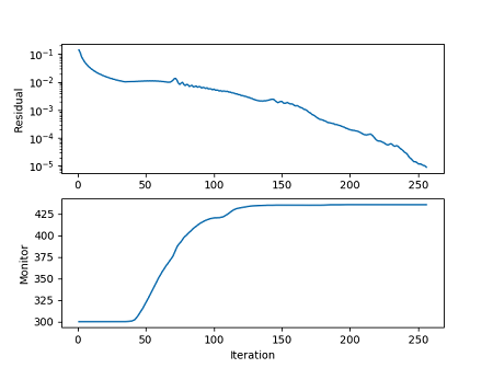
温度は150イタレーション以降はほぼ一定となり収束しているようです。このように、残差だけでなく目的の量の推移も合わせて見ていくとよいでしょう。

結果の温度コンター図は以下のようになりました。

2次元熱伝導の温度コンター図

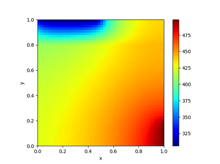
右下の500Kのところから左上の300Kの箇所へ徐々に温度が変化している様子がわかります。今回の条件では $y \ge 0.8$ で熱伝導率が小さいため、温度の低い箇所はその領域に抑えられています。

このプログラムを少し変更すれば、境界条件を変えたり、違う熱伝導率の組み合わせで計算することができます。また、発熱量 qc を与えると発熱を伴う計算も行うことができます。以下の結果は中央付近に2箇所発熱を与えた場合の例です。

発熱がある場合の温度分布

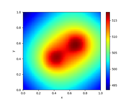
他の条件でもいろいろ計算してみてください。

まとめ

今回のシリーズでは、2次元熱伝導方程式をシミュレーションするプログラムを作りながら、有限体積法について学びました。有限体積法がどのような手法なのか理解できたでしょうか。

流体解析に適用したり、多様な形状のセルを使ったり、非定常問題を解いたりするためには、さらに複雑な定式化やスキーム、解法などが必要になります。また、計算速度を高速化したり、大規模な問題に適用したりするためには、データの格納方法や参照方法、他のアルゴリズムやプログラム言語を考える必要も出てきます。ただ、有限体積法をざっくり把握するには、ひとつの取っ掛かりになったのではないかと思います。

汎用の解析ソフトを使うにしても、その中でどのような手法で解かれているかを知っておくのは役に立ちます。「残差」とか「メッシュ」とか「解法」とか、言葉をブラックボックスにしておくより、きちんとイメージできていた方が解析やシミュレーションの仕事の助けになるかもしれません。

流体解析もまた機会があれば書いてみたいと思います。


←前回 共役勾配法で線形方程式系を解く

全体の目次

スポンサーリンク
科学技術計算のご相談は「キャットテックラボ」へ

科学技術計算やCAEに関するご相談、計算用プログラムの開発などお困りのことは「株式会社キャットテックラボ」へお問い合わせください。

お問い合わせはこちら

フォローする